9 minutes
Paper Summary: ControlNet
I recently hosted a remarkable paper group that explored the modifications to Stable Diffusion called “ControlNet.” Amidst the overwhelming spotlight cast on ChatGPT, it’s discouraging how quickly this model has receded from view. I think this is because most people are aware of the complexities of generating written content, but unaware of the challenges in image manipulation – and they are quick to dismiss imperfect AI-generated images. In reality, image manipulation is equally challenging.
Despite the prevalence of Transformer models, studying diffusion models remains valuable. I believe this for a few reasons:
- In contrast to the simple, repeated attention module underlying Transformers, Stable Diffusion has a very heterogenous structure and a complex interplay of several models and algorithms. With Transformers, the answer to “how can this be improved” is generally “add more data”; with Stable Diffusion, the field is much more fertile for fundamental research and improvements
- Stable Diffusion can model a stunningly complex generative distribution with a fraction of the parameters used in modern language models
- The terminology comes from an alternate universe of physics and it’s interesting to see deep learning through a novel lens
In this post, I share my insights from presenting the ControlNet paper: Adding Conditional Control to Text-to-Image Diffusion Models.
Prompts and control
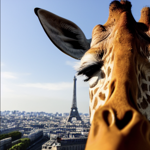
Stable Diffusion is prompt driven. If you ask for a photo of a Giraffe taking a selfie in Paris, you get this:
The model is “steerable” by injecting the prompt into the denoising U-net that lies at the core of the model. Specifically, the model is conditioned on a vector-embedded text prompt and a vector-embedded time step. (We use the term “time step” instead of, say, “progress” as a reference to the physics/differential equations literature from which the algorithm was inspired.)
In fact, if you look at the code, the injection is pretty clearly laid out. ResNet blocks incorporate the time information and vision transformers incorporate the prompt information. Each encoder/decoder block is composed of a vision transformer sandwiched between two ResNets. That super-block is repeated twenty-four times with residual links between encoder and decoder blocks with the same dimensions. Voila! That’s pretty much the entire architecture of Stable Diffusion.
Now, this model gives us control over what the image is about. But it doesn’t allow us to choose how to get there.
How to tell your model what you want
Let’s set a challenge for ourselves. We want the same image of the giraffe as above, but at night.
There are many ways to approach this problem, but one way might be to use a model that preserves the edges of the image.
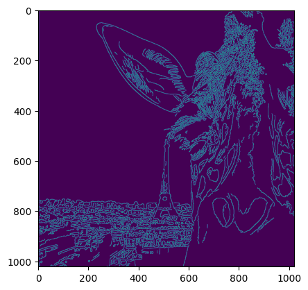
What do I mean by edges? I mean that in terms of the canny edge detection algorithm. For those unfamiliar, imagine fitting a spline to a black and white version of the Giraffe image. Then, imagine (1) applying a smoothing filter; (2) taking the partial derivatives of the spline with respect to $x$ and $y$ and; (3) taking the average of the partial derivatives. It looks like this:
import numpy as np
from skimage import feature
import matplotlib.pyplot as plt

img = Image.open("./giraffe.png").convert("L")
img = np.array(img)
edges = feature.canny(img)

plt.imshow(edges)
What if I told you that, after generating the image of the giraffe at night, the edges are preserved? That’s the promise of ControlNet.
I ran the original image through The Last Ben’s fork of Automatic1111 (which makes it easy to download the ControlNet weights).
And here it is.
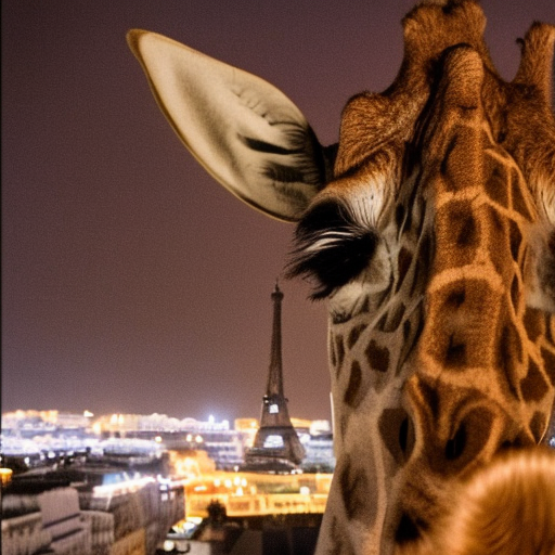
So cool! 😎
Edges aren’t the only way to control the model. In principle, any image transformation can work. The authors also trained models to incorporate the following conditioning information:
- Hough lines
- User scribbles
- Holistically-Nested edges
- Poses (openpifpaf and posenet)
- Segmentation maps
- Normal maps
- Monocular depth
So, how does it work?
ControlNet, as a kind of generic model modification
ControlNet refers to both the specific modifications to Stable Diffusion and a kind of architectural modification in general. That general modification looks like this:
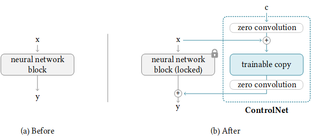
On the left, you have an arbitrary, pretrained neural network block. On the right, you have the original block – whose weights have been frozen – and a “trainable copy” with additional inputs.
from copy import deepcopy
from torch.nn import Module


class ControlNetBlock(Module):
    def __init__(self, original_block):
        super().__init__()
        self.original_block = original_block
        self.trainable_block = deepcopy(original_block)

        for param in self.original_block.parameters():
            param.requires_grad = False

        # ...snip
The inputs and outputs of this new path have a “zero” convolution layer. This is just a $1 \times 1$ convolutional neural network with the weights and biases initialized to zero.
class ZeroConv(Module):
    def __init__(self):
        super().__init__()
        self.conv = Conv2d(1, 1, kernel_size=1)
        self.conv.weight.data.fill_(0)
        self.conv.bias.data.fill_(0)

    def forward(self, x):
        return self.conv(x)
An aside: did you know that you can calculate a backwards gradient into a term that does not contribute to the output at all? My initial reaction was: if there is no contribution to the output, the gradient with respect to the term’s parameters is also zero and this network cannot be trained. Not so! All that matters when updating a functions parameters $F_\theta(X)$ is the derivative $\frac{\partial F}{\partial \theta}$, not the function output itself (whatever it may be). More explanation in the Github repo’s FAQ.
By “zeroing-out” the input to this module, the module gradually learns to pass information downstream into the network. Notice that, at first, this module has no contribution to the network at all. This is important during the training dynamics of ControlNet such that the normal Stable Diffusion process works without modification.
Notice that there are two trainable ZeroConv layers.
class ControlNetBlock(Module):
    def __init__(self, original_block):
        super().__init__()
        # ...snip
        self.zc1 = ZeroConv()
        self.zc2 = ZeroConv()
Moving on, notice that there is a new conditioning input, $\vec{c}$. This is the transformed image we discussed earlier, albeit projected into a smaller, latent subspace. (This is similar to the VAE used with Stable Diffusion, but it is just a small fully-convolution model they call $\varepsilon$). This projection is important because it squeezes the image into the $64 \times 64$ sized feature maps that Stable Diffusion expects.
That new conditioning input is passed through the zero-conv layer and added to the original latents. This sum is passed through the trainable copy of the stable diffusion block, which is then zero-conv’d once more. Finally, this output is added back to the output of the original stable diffusion block run against the original latents. This sounds more complicated than it is.
def forward(self, x, c):
    y_orig = self.original_block(x)
    xc = x + self.zc1(c)
    xc = self.trainable_block(xc)
    yc = self.zc2(xc)
    return yc + y_orig

ControlNetBlock.forward = forward
That’s pretty much it. If you ran that code, you would get the original model outputs. It only gets interesting once we train it, when $y_c \neq 0$. We’ll get to training in a moment.
ControlNet, applied to Stable Diffusion
The above description is overly simple for how the authors applied it to Stable Diffusion. Here’s how it actually looks:

This is the complete diagram of ControlNet, including details about Stable Diffusion.
Stable Diffusion is on the left. There are four information flows:
- From the top-down, the input latents are compressed into a $8 \times 8$ feature map space and decompressed into the original $64 \times 64$ feature map space
- From the left, the prompt embedding and the “time” embedding are incorporated into each of the blocks
- Also from the top-down, from encoder-blocks to decoder-blocks with the same dimension, residual links help pass along positional information
ControlNet adds an additional information flow, from the right:
- The conditioning vector $\vec{c}$ is mixed with the input latents and passed down to the middle block
- The output of each block is zero-conv’d and added to the appropriately sized decoder block
Note that the ControlNet blocks only add information to the normal flow of Stable Diffusion. That means you can add as many “control units” as you like. Each unit acts as a hyper-network, modifying the normal flow of Stable Diffusion for whatever conditioning vector.
What’s the point?
Why go through this effort to add zero-convolution blocks? Why not just add additional dimensions to the input latents and fine-tune?
Well, the authors were concerned about catastrophic forgetting. This is when fine-tuning on a few examples causes the model to lose the circuits that allow it to be capable under other domains. By freezing the original weights, and forcing the model to learn to only inject new information, the model doesn’t forget.
This also opens up the door to multiple conditioning, and the applications are quite interesting. Here’s a paper that improves temporal coherence of pose-retargeting by using two control net units: one for the target and another for the background.
Honestly, this line of reasoning is just speculation on my part. They do not provide convincing ablation studies, so its hard to compare to other approaches like fine-tuning. Nonetheless, the results speak for themselves.
Training
Amazingly, ControlNet does not require major modifications to the overall training regime. It is trained to gradually denoise images from the internet using the prompt and – now – the conditioning vector.
I assumed there would be some regularization loss to encourage the network to maintain edges or poses or whatever modality its trained on. Nope. It’s just continuous denoising, as per usual. This is a stunningly unexpected result.
The most interesting figure in the paper is Figure 21.
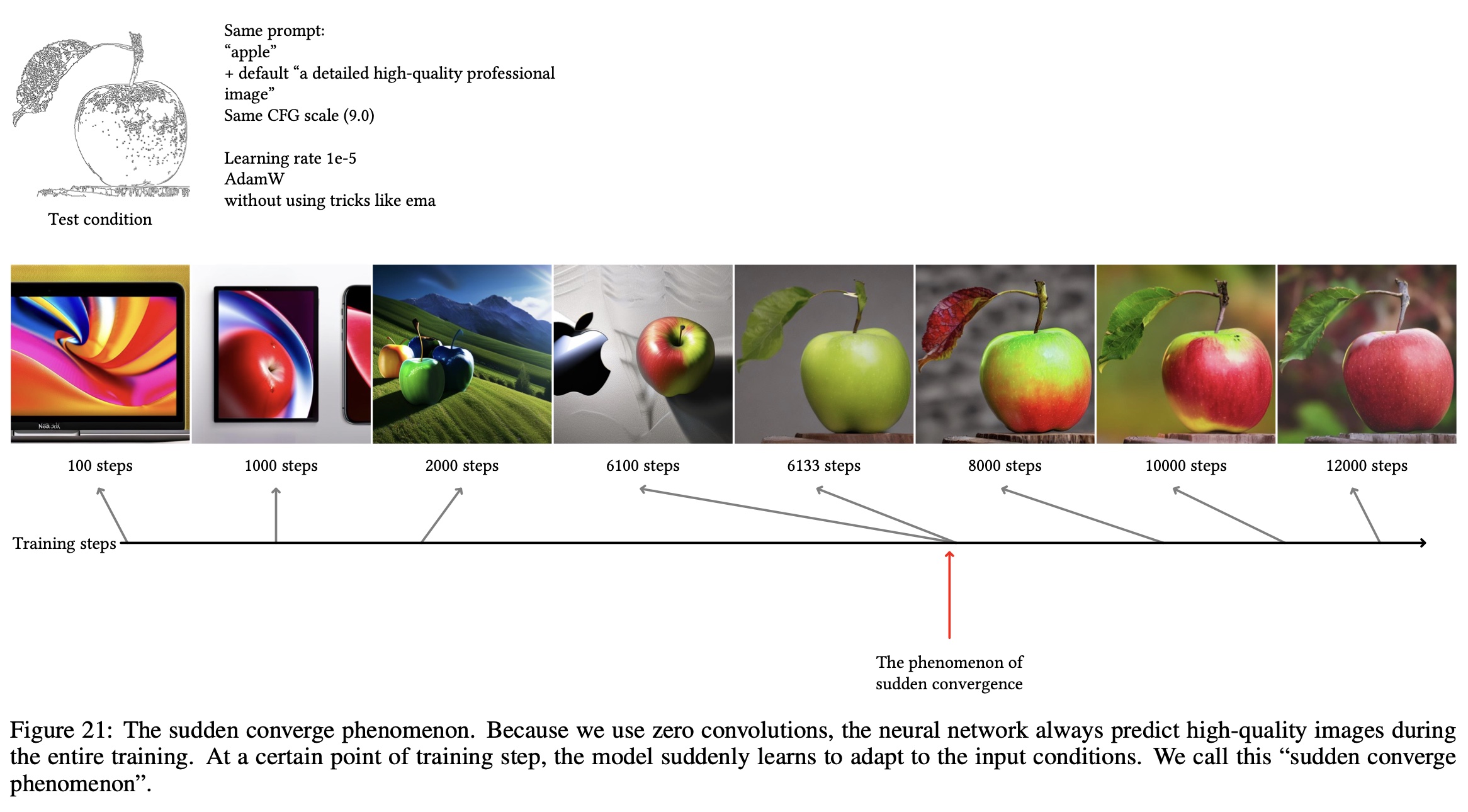
The canny-filtered apple is the conditioning vector and the series of images represents sampling at different stages of training. At approximately 6000 steps, the model begins to incorporate the conditioning vector consistently.
To me, this sounds pretty slow. Perhaps because the conditioning information is zero’d out so many times, it takes a while for any information from it to percolate up to the output.
Regardless, training is not the effective bottleneck. Once trained, inference is quick, as it will only have $1.5 \times$ the number of parameters compared to the base stable diffusion.
What does the future hold?
I expect that photo-manipulation software and game engines will eventually incorporate this model, specifically. It enables unprecedented precision with graphical manipulation. Imagine fully realistic skin and hair shaders, perhaps running real-time, without highly-tuned and expensive shader programs. This is speculation, of course: however, the underlying model is already extremely fast (it runs on a phone) and we will undoubtedly see it get even faster as distilled models become available and hardware specializes to serve it. The fact that they trained a model on normal maps is especially intriguing and suggestive of where things are heading.
Of course, any software that’s extremely capable like this can also be used for propaganda, misinformation, espionage and fraud. This will be a large and important use-case to be aware and wary of.
Personally, I am excited to see where this goes while also feeling caution and trepidation about the meaning and consequences of success in advancing the field of photo-manipulation.
1793 Words
2023-07-04 19:00