10 minutes
Notes on self-attention
As soon as I found out that OpenAI charged for input and output tokens, I realized that my understanding of self-attention needed some tweaking. I used to think that the input sequence was always padded or cropped to fit inside the context window, and that the length of the input sequence had no effect on the overall number of computations involved in running a transformer. But, I was wrong! (Apologies to the people I’ve misled when I’ve tried to explain this stuff in the past 😅)
This realization prompted me to embark on a project this week: implementing an autoregressive transformer by following Karpathy’s excellent video. Self-attention has a number of subtleties that need to be understood before we can appreciate its strengths. Essentially, any deep-learning-based sequence model must tackle the challenge of automatically learning useful syntactic and semantic features that arise from combining tokens, given a token sequence of length $T$, each with a feature vector with $C$ dimensions.
Consider the word “love” and its various shades of meaning depending on its context:
- I love mischief and deceit
- I don’t love chocolate cake
- I love you, but I’m not in love with you
To capture these nuances and their interplay with neighboring words, an ideal model needs to have a robust understanding of each token’s relationship with every other token.
So, let’s dive deeper into how self-attention works, why it’s more computationally expensive to process longer sequences, and how desirable properties emerge.
How self-attention works
At the heart of every transformer model lies the self-attention block. This block is responsible for allowing tokens to communicate with one another and compute combination-aware features while maintaining the tensor’s shape. (Maintaining the shape allows the operation to be repeated.) But how does it achieve this?
Well, it all starts with a simple mathematical trick. We begin with a matrix $X$ and perform the operation $\left( X \cdot X^T \right) \cdot X$, which allows feature vectors to interact with one another and reshapes the output appropriately.
What do I mean by “feature vectors interacting with one another”? I simply mean that there is some way for information to mix, in this case: by taking the dot product of the vector of continuous features of each token with the vector of every other token.
But there’s a catch: the computed features cannot be expected to be statistically important because this operation is non-parametric.
So, how do we make the computed features statistically meaningful? By adding a learnable, linear projection to each of the terms, like so:
$$ \left( XK \cdot ( X Q )^T \right) \cdot XV $$
Here, the linear projections are square matrices of rank $C$, which ensures that the shape of the tensor doesn’t change, and we end up with a $T \times C$ tensor in the end.
But wait, there are two critical modifications we need to make to this expression to get the desired self-attention behavior. The first is the softmax function, which converts the left-hand side of the expression into the “affinity” matrix. This matrix can be thought of as the weights in a weighted average of $X \cdot V$. The second modification is the causal mask, which ensures that the network only attends to tokens in the past. We achieve this by filling in the upper, off-diagonal elements of the pre-softmax attention matrix with $-\infty$, effectively forcing future weights to be zero.
You might be wondering how filling in $-\infty$ forces future weights to zero. This is subtle, so I’m including an example. Suppose we start with the following logits and learned weights $K$, $Q$ and $W$.
t, c = 3, 4
logits = np.random.rand(t, c)
k = np.random.rand(c, c)
q = np.random.rand(c, c)
v = np.random.rand(c, c)
np.round(logits @ v, decimals=2)
array([[1.36, 1.2 , 1.5 , 1.8 ],
       [0.26, 0.35, 0.27, 0.54],
       [0.65, 0.74, 0.93, 1.2 ]])
This produces an affinity matrix like so:
affinity_scores = (logits @ k) @ (logits @ q).T
affinity = scipy.special.softmax(affinity_scores, axis=1)
np.round(affinity, decimals=2)
array([[0.66, 0.03, 0.3 ],
       [0.52, 0.11, 0.37],
       [0.63, 0.04, 0.33]])
Suppose we were to use those logits – without a mask – to create a probability distribution, à la BERT. Let’s consider how to calculate the first channel of the output token of the attention layer. This is the dot product of the first row of the affinity matrix and the first column of the values matrix.
The meaning of the columns of the $V$ matrix is somewhat obtuse: each column has a size of $T$ and each value represents a statistically-derived continuous feature of the input token. For instance, the $i$th element of this column is a feature of the $i$th token.
The meaning of the rows of the affinity matrix are more straightforward: if we imagine the whole dot-product as a weighted average, then the affinity matrix rows are the weights. (Note that the sum of each row of the affinity matrix sums to $1$.)
In all, we get this:
$$ [0.66, 0.03, 0.3 ] [1.36, 0.26, 0.65]^T = 1.11 $$
One more point to make before we point out the problem with not including the attention mask. Consider the objective function of a sequence transducer: we need to predict a shifted version of the the input. Every token should be statistically transformed into the next token in the sequence. This is a lightly modified version of the input-output pair generation code in Karpathy’s video.
def get_batch(X):
    ix = torch.randint(len(X) - block_size, (batch_size,))
    x = torch.stack([X[i:i+block_size] for i in ix])
    y = torch.stack([X[i+1:i+block_size+1] for i in ix])
    return x, y

xb, yb = get_batch(X_trn)

for t in range(block_size):
    context = xb[0, :t+1]
    target = yb[0, t]
    print(f"{decode(context)}: {context.tolist()} -> {target} ({decode([target])})")
L: [24] -> 43 (e)
Le: [24, 43] -> 58 (t)
Let: [24, 43, 58] -> 5 (')
Let': [24, 43, 58, 5] -> 57 (s)
Let's: [24, 43, 58, 5, 57] -> 1 ( )
Let's : [24, 43, 58, 5, 57, 1] -> 46 (h)
Let's h: [24, 43, 58, 5, 57, 1, 46] -> 43 (e)
Let's he: [24, 43, 58, 5, 57, 1, 46, 43] -> 39 (a)
This provides an obvious way for the network to converge on a useless algorithm. That is, each token can simply copy the information from the token to its right. In essence, the ideal weighted sum from earlier look like this:
$$ [0, 1, 0] [1.36, 0.26, 0.65]^T = 0.26 $$
And the ideal affinity matrix looks like this:
$$
\begin{bmatrix}
0 & 1 & 0 & 0 \\
0 & 0 & 1 & 0 \\
0 & 0 & 0 & 1 \\
? & ? & ? & ?
\end{bmatrix}
$$
That results in a perfect solution for every token except the last one, where you can’t do this trick. Of course, this is the only token that matters because its what we use during inference. Therefore, this “trick” is counterproductive.
We can solve this by forcing the weights to fall on tokens that are in the “present” or “past” from the perspective of the output token. By setting the upper-right of the affinity scores to $-\infty$ and taking the row-wise softmax, we simply ignore the weights from tokens in the future. Simply note that $e^{-\infty}=0$ and the final weights are distributed among the past and present tokens. Thus, for our example:
masked_affinity_scores = affinity_scores[:]
masked_affinity_scores[np.tril(np.ones((t,t))) == 0] = float("-inf")
np.round(masked_affinity_scores, decimals=2)
array([[5.17, -inf, -inf],
       [2.78, 1.22, -inf],
       [4.73, 2.  , 4.07]])
Applying the softmax:
affinity = scipy.special.softmax(masked_affinity_scores, axis=1)
np.round(affinity, decimals=2)
array([[1.  , 0.  , 0.  ],
       [0.83, 0.17, 0.  ],
       [0.63, 0.04, 0.33]])
Gives us the weights for the first channel:
$$ [1, 0, 0] [1.36, 0.26, 0.65]^T = 1.36 $$
Thus, the network is constrained to pull information from the past and present. In this case, the first channel of the first output token is a function of the first channel of the input token, because it cannot pull information from anywhere else. The first channel of the output token of the second token can, however:
$$ [0.83, 0.17, 0] [1.36, 0.26, 0.65]^T = 1.173 $$
Pretty cool, if you ask me 😁
And that’s how self-attention works in a nutshell! Of course, this explanation doesn’t cover all the details of multi-headedness, attention-scaling, residual connections, normalization, dropout, and the feed-forward networks. But hopefully, it gives you a good idea of the key ideas behind self-attention.
Why it’s more computationally expensive to process longer sequences
This explanation reveals why longer inputs are more computationally-expensive for longer sequences: because the $K \cdot Q$ calculation grows quadratically in computationally complexity with the size of the $T$ dimension (i.e., the number of tokens in the sequence). This suggests that the attention-score calculation is the computational bottleneck for transformers.
But is this the whole story?
Consider this excellent article on how GPT-3 spends its 175B parameters. Here’s how different formulations of GPT-3 have their parameters allocated:
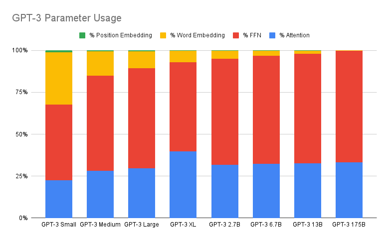
Less than a third of the parameters in these models are allocated to the self-attention layer. I’ve heard rumors that the proportion of parameters allocated to self-attention in larger models like PaLM is even less.
One of the points I set out to make when I began this post is that the complexity analysis is misleading: that, in fact, the majority of processing on these models is done in the feed-forward layer. However, I am unable to find written evidence for this argument, since it depends on the length of the sequence. Moreover, in my experiments, I found that using the built-in, fused scaled dot product attention operator in Pytorch was almost twice as fast to train compared to my naive implementation. This is strong evidence that, indeed, attention is likely the computational bottleneck for transformers.
Additional properties of Transformers that makes them scalable and also good
To sum up, self-attention is a statistical transformation that comes with some pretty sweet bonuses. Unlike feed-forward networks, which have strong translational-equivariant bias, self-attention is flexible and can preserve or ignore positional information, as needed.
Furthermore, separating the “attention” calculation from the “value” calculation allows the model to pass along statistical patterns from the input in a way that’s tailored to the task at hand. This is called the “data-specific kernel” property.
While both properties afford the model flexibility, it’s not clear why flexibility improves the modeling performance. Generally speaking, algorithms converge only when their priors match the symmetries of the data. But transformers don’t really have strong priors. So, the community consensus about self-attention is that the excellent modeling performance of transformers is an empirical result, rather than a theoretical one.
However, it does feel intuitive that transformers represent language more robustly than anything we’ve had before in deep learning and computer science. Compare to earlier approaches:
- RNNs/LSTMs compress past language into a “latent” vector and learn a conditional probability distribution for the next word in the language
- Phrase structure grammars build rulesets underlying words that govern acceptable continuations
Neither of these seems to be related particularly to my own experience of consciousness: I don’t think in terms of a vector-memory and I only vaguely concern myself with grammar or parse trees. My own experience of language production is (I) drawing upon my recent memory of the past, (II) groping for the next word in the present and (III) planning in the near future to express certain, pre-language “intentions” that I am only aware of once I have summoned the words for them into existence. Transformers feel well-suited for this because build these combinatorial, semantic features over sequences from past and presently-produced language all at once. Then, they sample words one at a time. This feels right.
In any case, what’s certain is this: among sequence transducers, transformers are uniquely efficient to train on a GPU, as they can backpropagate through an arbitrarily long sequence with a single pass through the network. This is in contrast to recurrent neural networks, which require a forward propagation for each input and output token, making transformers an order-of-magnitude quicker to train. (Check out this video where Vaswani makes this point.) This, more than anything, is the characteristic that makes Transformers so pervasive in real-life. Training more quickly enables scale and machine learning works at scale. The advantages of Transformers from a modeling are widely exaggerated; their chief advantages derive from favorable performance on accelerated hardware.
In summary, the beauty of transformers lies in their ability to satisfy the constraints of a sequence transducer while enabling scale in terms of the amount of data they can store and process. They also, possibly, recapitulate a more realistic model of intelligence.
2096 Words
2023-04-01 19:00