15 minutes
Scaling up Transformer training on a shoestring
Once you have a machine learning pipeline that works well on a small dataset, how do you scale it to fit larger models on more data, faster? It requires a finely-tuned data loading strategy and model architecture, a grasp of scaling dynamics, and a GPU cloud setup. I’ve honed my own skills training a GPT3 small model on English wikipedia with PyTorch. Here are my findings and recommendations.
Fast data loading
A common bottleneck in model training often stems from sluggish data loading practices. Consider the widespread use of Pandas, for instance, and how it not only results in excessive memory consumption but also poses challenges in designing more efficient alternatives.
Frequently, data scientists craft Python scripts that locally load and transform data, followed by the creation of a dataset wrapper class. Take, for example, the following Pandas-based implementation:
from .utils import preprocess

class PandasDataset(torch.utils.data.Dataset):
  def __init__(self, df):
    self.df = df

  def __len__(self):
    return len(self.df)

  def __get_item__(self, idx):
    row = self.ds[idx]
    row = preprocess(row)
    return {“results”: “row”}

df = pd.read_csv("foo.csv")
ds = PandasDataset(df)
This approach has two serious, non-obvious constraints:
- Its memory consumption can be 2-10 times larger than on-disk consumption, as elaborated here.
- Lack of shared memory semantics in Pandas means that multi-processing requires a full copy of the data for each process.
Consider a scenario where the preprocess function is embarrassingly parallel, and 8 workers are assigned to perform the computation as data is fed to the model.
train_dataloader = DataLoader(
  PandasDataset(df=pd.read_csv("train.csv")),
  batch_size=64,
  num_workers=8,
)
Each worker, in this case, creates a copy of its state, resulting in a 10x overhead for a 2Gb CSV file, ultimately requiring 160 Gb RAM. On Google Compute Engine, an n1-standard-64 instance with 4x T4 GPUs instance satisfies this memory requirement with 240 Gb RAM at \$3.11 hourly. By avoiding this memory-intensive process, one can opt for a more cost-effective instance, such as an n1-standard-4 with 15 Gb RAM at $1.11 hourly, resulting in a 64% cost savings with a straightforward code change.
To overcome these limitations, it’s crucial to avoid passing the data into the Dataset object before loading it into a Dataloader. Consider passing a reference to the data and loading it lazily, as shown below:
import torch
import json
import smart_open

from .utils import chunkify, preprocess

class LazyShardedDataset(torch.utils.data.IterableDataset):
  def __init__(self, shards):
    self.shards = shards

  def __iter__(self):
    wi = torch.utils.data.get_worker_info()

    if wi is not None:
      worker_shards = chunkify(self.shards, nchunks=wi.num_workers)[wi.id]
    else:
      # Single-worker or same process as the training script
      worker_shards = self.shards

    for shard in worker_shards:
      with smart_open.open(shard, "rt") as f:
        for line in f:
          row = json.loads(line)
          # Perform on-the-fly computations
          row = preprocess(row)
          yield row

ds = LazyShardedDataset([
  "gs://mydata/shard1.jsonl",
  "gs://mydata/shard2.jsonl",
  "gs://mydata/shard3.jsonl",
])
This approach bypasses Pandas’ performance limitations by holding only the mini-batch in memory, minimizing the memory footprint, and dispatching different shards to independently operating workers, thus removing the coordination burden.
While the provided example is effective, for more flexibility and maturity, consider exploring Huggingface’s datasets library, which offers streaming, lazy/on-the-fly processing, pre-processing, test-train split saving, mmap, and more. Additionally, MosaicML streaming is a viable option that also provides resumability, a topic we’ll delve into in the section on distributed training.
Given that GPUs are a significant cost in the machine learning pipeline, performance-tuning data preprocessing is essential to ensure these machines can swiftly churn through data as soon as they are ready.
Model implementation
Kernel fusing
Performance can also be impacted by the model implementation itself. Generally speaking, condensing the forward-backward propagation cycle into as few operations as possible also minimizes costly memory IO.
For example, self-attention is mathematically represented as five matrix products per head, as well as one additional product for re-weighting the heads (see section 3.3 of the Attention Is All You Need paper). To be specific, three of those operations project the input logits into the head’s key, query and value spaces, respectively. Then, for each head, the $K$ and $Q$ matrices are multiplied to produce the affinity matrix (They have a scaler, mask, softmax and dropout layer applied as well; but we’ll focus on matrix products here). Finally, the head’s affinity matrix is multiplied with the head’s $V$ matrix. GTP3-small has twelve heads, so this entails 61 matrix products per attention layer.
Can we reduce this number? Indeed, multi-headed self-attention can be expressed as just four matrix products, regardless of the number of heads, like so:
Compute $K$, $Q$ and $V$ projections for all heads simultaneously:
kqv = nn.Linear(768, 3 * 768)
x = kqv(x)
Rearrange the combined matrix with a new axis representing the head index, and a new axis representing $K$, $Q$ or $V$. Then, compute the affinity scores. (Recall that einsum is a matrix product when input axes are dropped on the right-hand side; in this case, note that the channel dimensions
hsaandhsbare dropped.)k, q, v = einops.rearrange( x, "b t (s nh hs) -> s b nh t hs", s=3, nh=12, hs=768 / 12, ) affinity_scores = einops.einsum( q, k, "b nh ta hsa, b nh tb hsb -> b nh ta tb", )Apply the causal mask, etc (omitted). Compute the product of the affinity matrix and the $V$ matrix.
x = affinity @ vConcatenate and reweight the heads
x = einops.rearrange(x, "b nh t hs -> b t (nh hs)")
W = nn.Linear(768, 768)
x = W(x)
On my Nvidia 3090, using this implementation compared to a naive one increased training speed by 20%. It can be improved further by using the new torch.nn.functional.scaled_dot_product_attention. By combining this improved implementation and the fused attention module, I achieved a speed up of 550%. Not bad 😄
In theory, the new torch.compile API should also improve speed by automatically combining operations, but I found it reduced training speed by 7% – even with the reduce-overhead option.
Running these experiments on a smaller, cheaper machine gave me confidence that I was maximizing utility when I rented out a much larger, more expensive instance later on.
Distributed execution
The final component of an efficient training workflow is the efficient utilization of multiple GPUs. This requires a clear understanding of the distributed training algorithm, with Distributed Data Parallelism (DDP) being the most prevalent.
I am going to use parallel computing terminology here. A “world” is a process group, where each process controls an individual GPU. The “world size” is the number of processes. The “local rank” describes the index of the process within the world, as well as the process itself.
Briefly, the algorithm accomplishes the following for each forward-backward propagation cycle:
- Individually, each local rank process receives identical model weights and a different data batch
- Individually, each local rank process conducts a forward propagation and computes the loss and parameter gradients
- Altogether, the world determines the average loss and average parameter gradients
- Individually, each local rank executes a back-propagation pass, leading to synchronized, updated weights
What is often ignored or misunderstood is that each process is running the exact same python code as the parent process (i.e., the “rank zero” process), with most of the same command line arguments. The only difference is the LOCAL_RANK environment variable, which is set to a number from 1 to the world size. If misunderstood, either:
- code will execute once per-GPU that should be run once overall, like logging and saving weights
- the rank zero process will hang indefinitely as it waits for a synchronization signal that never arrives
PyTorch Lightning serves as an organizational framework for PyTorch and helps, among other things, streamline code for distributed scenarios. By adopting its semantics, logging and model checkpointing should work as expected and only run on the rank-zero process. Others, like the Weights and Biases logger, requires additional safeguards. Using the wandb logger as an example, something like this would start one run per GPU:
import wandb
import torch
import pytorch_lightning as L

class MyModel(L.LightningModule):
  def __init__(self):
    super().__init__()
    self.l = torch.nn.Linear(1,1)
    self.criterion = torch.nn.MSELoss()

  def forward(self, x):
    return self.l(x)

  def training_step(self, batch, batch_idx):
    y = self(x)
    loss = self.criterion(y, 2*x)
    self.log("training/loss", loss)
    return loss

with wandb.init():
  model = MyModel()
  dataloader = ...  # Use your favorite data here
  trainer = L.trainer()
  trainer.fit(model, train_dataloaders=dataloader, accelerator="auto")
To discard the useless, extra experimental runs in the Weights and Biases interface, we need to avoid initializing wandb on non-rank-zero processes like so:
import wandb
import torch
import pytorch_lightning as L
import os
import contextlib

def get_rank_zero_or_single_gpu():
  """Return whether the current process is the rank zero process."""
  return os.environ.get("LOCAL_RANK", "0") == "0"

@contextlib
def wandb_init():
  if get_rank_zero_or_single_gpu():
    with wandb.init():
      yield
  else:
    yield

class MyModel(L.LightningModule):
  def __init__(self):
    super().__init__()
    self.l = torch.nn.Linear(1,1)
    self.criterion = torch.nn.MSELoss()

  def forward(self, x):
    return self.l(x)

  def training_step(self, batch, batch_idx):
    y = self(x)
    loss = self.criterion(y, 2*x)
    self.log("training/loss", loss, sync_dist=True)  # 👈 notice the `sync_dist` argument
    return loss

with wandb_init():  # 👈 notice this uses the new context manager
  model = MyModel()
  dataloader = ...  # Use your favorite data here
  trainer = L.trainer()
  trainer.fit(model, train_dataloaders=dataloader, accelerator="auto")
Notice that we add sync_dist=True. This averages the loss from each process before logging it to the Weights and Biases system. We also add the context manager, preventing initialization of the extraneous runs on the other GPU’s. In all, these modifications prevent unintended log events and synchronizes the logged value appropriately. See the logger docs for more details.
The other class of error derives from code clobbering worldwide synchronization signals, leading to deadlocks. Again, using PyTorch Lightning as a starting point, this example code will hang indefinitely. This is because the rank zero process running on_train_epoch_end waits for the termination signal from the other processes running the method. However, the rank_zero_only decorator makes the method a no-op, preventing non-rank-zero processes from emitting the synchronization signal.
from pytorch_lightning.utilities.rank_zero import rank_zero_only
from .utils import report_metrics_to_server, expensive_once_per_epoch_computation

class MyModel(L.LightningModule):

	# snip...

  @rank_zero_only
  def on_train_epoch_end(self):
    report = expensive_once_per_epoch_computation(self)
    report_metrics_to_server(report)
This should be written like so:
class MyModel(L.LightningModule):

  # snip...

  def on_train_epoch_end(self):
    if get_rank_zero_or_single_gpu():
      report = expensive_once_per_epoch_computation(self)
      report_metrics_to_server(report)
The PyTorch lightning multi-GPU training docs are extremely useful. Make sure to carefully check all parts of the codebase that should be run only once, ensuring that they are guarded by an appropriate condition or decorator.
These are samples of the issues that crop up in the distributed setting that must be accounted for to ensure proper instrumentation and world-wide communication. It is essential to address them to allow scaling up from a single-GPU, which may contain tens of Gbs of vRAM, to multiple GPUs that collectively contain hundreds of Gbs of vRAM.
Choosing how to scale
How much data and how many parameters should your model have for a given budget? Training costs and inference costs must be considered holistically to make an informed decision.
As for training, the “Training Compute-Optimal Large Language Models” paper describes the relationship between data size, model size and model loss for Transformers. To determine this, DeepMind researchers trained hundreds of models with various sizes and budgets. (The dataset size was constrained to match the model’s processing capacity within the allocated budget; in other words, dataset size is a dependant variable, albeit one governed by a well-understood relationship.)
The results, depicted in the below figure, illustrate the covariance between loss (y-axis) and the number of parameters (x-axis) across different computational budgets (color). The surface resembles a slanted half-tube, with “Chinchilla-optimal points” representing the lowest loss for a given budget. Connecting these points forms a line.
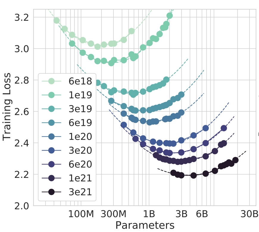
This finding forms the basis for their scaling recommendations: if aiming for a lower loss with a larger budget, increase model size and data size proportionally.
However, this “efficiency frontier” evaluated relatively small models from 100 million to tens of billions of parameters. Did this guidance hold for models well outside of the range considered? Was the curvature still linear? To determine if this was the case, they trained a 70 billion parameter model (which was ~3x bigger than the largest model considered in the study) on 1,400 billion tokens (which was larger than any dataset used to train a Transformer at that time). The resulting model, christened “Chinchilla,” outperformed “Gopher,” which was larger but trained on less data.
This wasn’t always the accepted wisdom for scaling. OpenAI published the “Scaling Laws for Neural Language Models” paper in 2020, which contended that optimal scaling was governed by a power-law relationship. That is to say: larger models were thought to be more sample efficient. Therefore, proportionally more compute budget should be allocated to the model size as the budget increases. I’ve read these papers many times, and I still failed to understand why the OpenAI paper was considered wrong until I read this blog post. The author does an excellent job explaining this discrepancy, and I’ll just quote it here.
Given the evidence of Chinchilla, it appears pretty definite that OpenAI got the scaling laws wrong. So one natural question is “What happened that they got it wrong?”
Well, background: The learning rate of a deep neural network dictates how much the parameters of a network are updated for each piece of training data. Learning rates on large training runs are typically decreased according to a schedule, so that data towards the end of a training run adjusts the parameters of a neural network less than data towards the beginning of it. You can see this as reflecting the need to not “forget” what was learned earlier in the training run.
It looks like OpenAI used a single total annealing schedule for all of their runs, even those of different lengths. This shifted the apparent best-possible performance downwards for the networks on a non-ideal annealing schedule. And this lead to a distorted notion of what laws should be.
This being said, Chinchilla-optimality is geared towards frontier lab researchers seeking to push model capabilities, prioritizing training costs over all else. This perspective neglects the inference cost consideration in machine learning products, where inference usually outweighs training expenses. For example, OpenAI spent $4 million to train ChatGPT and spends $700 thousand every day to serve it. It is widely suspected that, to reduce costs, OpenAI later substituted a smaller model to back ChatGPT. If they did so, they would have undoubtedly trained it on more data than suggested by DeepMind’s efficiency frontier. This is an important insight. Businesses will increasingly understand that deploying smaller models trained on more data is more cost-effective and practical.
You can listen to an excellent discussion of how MosaicML trained their MPT model with this insight in mind here.
Training remotely
While GPUs are abundant in production, consumer availability remains scarce. How can one rent powerful machines for short-term usage and make the most of the time?
I have personally had success with AWS Sagemaker and Vast.AI. I’ll share tips here for using VastAI effectively, since I find it a more pleasant alternative.
Docker deployments
Vast.AI supports deploying Docker images, which allows us to side-step the time-consuming task of downloading and compiling the deep learning stack. We wouldn’t want to rent a GPU-instance and waste time compiling code on it.
However, while Docker allows us to pre-compile, its build and run interfaces can be frustrating. Starting with an OS image like Ubuntu requires installing CUDA drivers, Python, Torch, and more. Questions arise: should we use miniconda and maintain a lockfile? Do we employ bind mounts or the ADD directive to add code? Ensuring efficient cache usage adds another layer of complexity. In essence, there are numerous decisions and engineering tasks before achieving even the simplest tasks using Docker.
Cog simplifies the process of writing and running dockerfiles, streamlining CUDA and Python installation and providing a simple interface to mount the current working directory. Configuration in Cog involves a cog.yaml file, like so:
build:
  gpu: true
  python_version: 3.10
  python_requirements: requirements.txt
predict: "gpt/predict.py:Predictor"
To use Cog, simply prefix your training command with cog run, and it utilizes a Docker container as if it were a local script. This doesn’t come without drawbacks. For example, only the current working directory is mounted, so directories like the Huggingface cache are not preserved between runs unless the script is adjusted to use the current working directory as a cache.
In my case, I used Cog solely to produce a Docker image for consumption on VastAI. This works extremely well because Cog configures the RUN cache for Python and Ubuntu by default. The RUN cache is distinct from the ubiquitous build cache: rather, this cache persists installation tool cache directories (e.g., ~/.cache/pip) between builds. This feature proves particularly beneficial in the context of Github Actions, which only supports a RUN cache. And, because pushing to Dockerhub is so fast, I was able to reduce the deployment time from ninety minutes to ten minutes.
Here is an example Github Action:
name: Push to DockerHub
on:
  push:
    tags:
      - "v*"
jobs:
  build:
    runs-on: ubuntu-latest
    steps:
      - name: Check out code
        uses: actions/checkout@v3
      - name: Login to Docker Hub
        uses: docker/login-action@v3
        with:
          username: ${{ secrets.DOCKERHUB_USERNAME }}
          password: ${{ secrets.DOCKERHUB_TOKEN }}
      - name: Setup Cog
        run: |
          curl -o /usr/local/bin/cog -L "https://github.com/replicate/cog/releases/latest/download/cog_$(uname -s)_$(uname -m)"
          chmod +x /usr/local/bin/cog
      - name: Push to DockerHub
        run: |
          cog push ${{ secrets.DOCKERHUB_USERNAME }}/my-docker-image:${{  github.ref_name }}
          cog push ${{ secrets.DOCKERHUB_USERNAME }}/my-docker-image:latest"
Then, I simply specify the docker image in the CLI and download the code in the “onstart” script.
vastai create instance $INSTANCE_ID \
  --image my-docker-image \
  --env "-e WANDB_API_KEY=$(jq -r .WANDB_API_KEY < .secrets)" \
  --disk 100 \
  --ssh \
  --onstart ./on-start.sh
# on-start.sh
git clone https://github.com/jeremyadamsfisher/shakespeare_transformer.git
cd shakespeare_transformer
export PYTHONPATH=$PYTHONPATH:$(pwd)
nohup python -O gpt/train.py +model_config=gpt3_small_char &
Resuming training
While my final training run did not crash, I did implement a pause-and-resume feature just in case. I used the PyTorch Lightning model checkpoint callback to save the model and optimizer states to Google Cloud Storage, and I saved the Weights and Biases run ID as part of the blob name.To resume training, I would have simply provided the run ID, allowing it to restore the state.
There are important caveats to consider when resuming from such a checkpoint. Once a training run begins, the dataloader adjusts the effective batch size based on the number of GPUs. However, the dataloader state only keeps track of the total number of batches, not which specific batches it has processed. Consequently, when resuming on a machine with a different GPU count, it may reuse or skip batches. This behavior is attributed to a limitation of PyTorch dataloaders. To address this challenge robustly, a solution like Mosaic Streaming is necessary, but beyond what I personally needed or implemented.
Conclusion
Training a GPT-3 class model is surprisingly accessible. Overcoming performance and infrastructure challenges is feasible, especially with platforms like Vast.AI. Whether deploying an Nvidia 4090 or eight A100s, boasting up to 640 GB vRAM, we’ve got a wide variety of scenarios covered. Follow the tips shared here to scale up efficiently, maximize the value of your cloud compute and train a large language model.
3132 Words
2023-11-24 17:02